Feeds:
Posts
Comments

Posts Tagged ‘vcf’

Autozplotter_mesut_erzurumluoglu

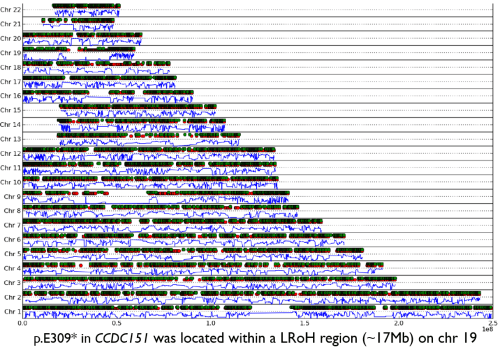
An example output from AutoZplotter using whole-exome sequencing data – used to identify the Primary ciliary dyskinesia causal gene, CCDC151, in Alsaadi and Erzurumluoglu et al, 2014 (read this paper’s story here). The green and red dots correspond to heterozygous and homozygous calls (for the alternative allele), respectively. The continuous blue lines correspond to the probability that the observed sequence of genotypes is not autozygous (e.g. close to zero means likely to be an autozygous region). LRoH: Long runs of homozygosity. NB: This image has been edited to ensure confidentiality/anonymity of the participant. Some LRoHs have been shortened or extended for this reason. If you’re thinking of using an AutoZplotter image in a paper, do not share genome-wide figures but maybe consider using chromosome-wide ones

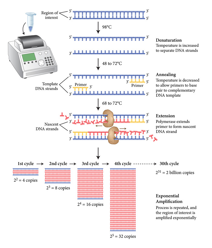
When analysing whole-exome or whole-genome sequencing (or dense SNP chip) data obtained from consanguineous individuals with a rare Mendelian disease, the disease causal mutation usually lies within an autozygous region (characterised by long runs of homozygosity, LRoH, which are generally >5Mb). Thus checking whether any candidate genes overlap with an LRoH can substantially narrow region(s) of interest. There are several tools which can identify LRoHs such as Plink, AutoSNPa and AgilentVariantMapper. However, they all require their own formats and considerable computational knowledge; and also struggle to identify regions that are shorter than 5Mb. Thus, we wrote AutoZplotter, a user-friendly python script which plots the heterozygosity/homozygosity status of variants in a VCF file to allow for quick visualisation and manual identification of regions that have longer stretches of homozygosity than would be expected by chance.

VCF_format_v4

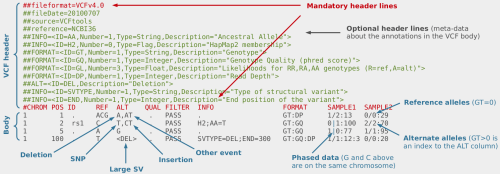
AutoZplotter accepts the VCF format – which is the standard format for storing genetic variation data from NGS platforms. Image Source URL: bioinf.comav.upv.es

The input format of AutoZplotter is VCF, thus it will be suitable for any type of genetic data (e.g. SNP array, WES, WGS) and from any species.

An older version of AutoZplotter was used in the analysis stage of Alsaadi et al (2012) and Alsaadi and Erzurumluoglu et al (2014).

To download latest version of AutoZplotter, click here (directs to ResearchGate). If you found AutoZplotter helpful in anyway, please cite Erzurumluoglu AM et al, 2015.


References:

Erzurumluoglu AM et al, 2015. Identifying Highly Penetrant Disease Causal Mutations Using Next Generation Sequencing: Guide to Whole Process. BioMed Research International. Volume 2015 (2015), Article ID 923491

Alsaadi MM and Erzurumluoglu AM et al, 2014. Nonsense Mutation in Coiled-Coil Domain Containing 151 Gene (CCDC151) Causes Primary Ciliary Dyskinesia. Human Mutation. Volume 35, Issue 12. Pages 1446–1448

Erzurumluoglu AM et al, 2016. Importance of Genetic Studies in Consanguineous Populations for the Characterization of Novel Human Gene Functions. Volume 80, Issue 3. Pages 187–196

Erzurumluoglu AM, 2015. Population and family based studies of Consanguinity: Genetic and Computational approaches. PhD Thesis. University of Bristol

Read Full Post »

Polymerase Chain Reaction (from www.neb.com)

Schematic of the PCR (Polymerase Chain Reaction) process – a technique used to amplify a specific region of DNA. Source URL: http://www.neb.com

This is a very quick guide to designing a primer for PCR (Polymerase Chain Reaction) which will be used to amplify a region of interest. The produced amplicons can then be sent to companies such as GATC-Biotech (located in Germany) to be sequenced. I have seen many blogs with this title but none of them guide you in the way you would expect them to. So I decided to write my own to hopefully make things easier for you:

(i) To design a primer, first click on the link below:

Primer Blast

(ii) On the Primer Blast page, you will come across the ‘PCR Template’ box at the top. Enter the ‘Accession ID’ of your transcript of interest from RefSeq if you’re working with mRNA.

If you’re interested in amplifying a genomic region then use Ensembl by (i) searching for your gene of interest on the Ensembl homepage; (ii) then clicking on your gene of interest in the results; (iii) then in the ‘Gene’ view, clicking on the ‘Sequence’ in the ‘Gene-based display’ on the left; and (iv) then by copying the ‘Marked-up sequence’ in FASTA format and pasting it into the ‘PCR Template’ box.

Calculate where your variant of interest is located in the FASTA sequence (Ensembl) or in the transcript (RefSeq mRNA) you pasted and fill in ‘Forward Primer’ and ‘Reverse Primer’ accordingly. I’d advise having a flanking region of ~150bp on both sides of your variant (e.g. if your variant is located at position 500 in your FASTA sequence, then type 350 into ‘From’ in ‘Forward Primer’ and 650 into ‘To’ in ‘Reverse Primer’, leave the other two empty).

(iii) In Primer Parameters:

To get the amplicon sent and sequenced at a company, keep the PCR product size manageable (e.g. 150bp to 300bp).

(iv) If working with human genomic data, change ‘Database’ to ‘Genome (reference assembly from selected organisms)’ and select ‘Homo sapiens’ as ‘Organism’ in ‘Primer Pair Specificity Checking Parameters’.

Click ‘Advanced parameters’.

(v) Change ‘Primer Size’ in ‘Primer Parameters’ to 18 (min), 22 and 25 (max) respectively.

Change ‘Primer GC Content (%)’ to 40.0 and 60.0 respectively.

Change ‘GC Clamp’ to 1.

Change ‘Max Poly-X’ to 3.

Tick the ‘SNP handling’ box (important!).

(vi) Scroll to bottom and click ‘Show results in a new window’ before clicking  ‘Get Primers’.

(vii) Wait for results and select a couple* of primer pairs and test them in an in-silico PCR software (e.g. UCSC In-Silico PCR) – designing at least two primer pairs is important; in case one fails, the other one usually works.

(*check that the GC content of the forward and reverse primers are similar to each other for each primer pair.)

Once you’re happy with the amplicons produced in the in-silico PCR program (e.g. your variant** of interest is located towards the centre of the amplicon as desired) then check for hairpin formation (both for forward and reverse primer, separately) using a software such as OligoCalc.

(**if your gene of interest is on the reverse strand, then you would have to use software such as Reverse Complement to change the sequence of your amplicon to its complement so that it matches the Ensembl gene sequence that you’re comparing it against – where you obtained the sequence in FASTA format in step ii).

Once your primer pairs pass all these tests, order them from a company such as Eurofins.

When performing PCR, choosing the annealing temperature may not be straightforward. Although there is a formula for calculating optimum annealing temperature (Ta; see link), (for primers with no unintended targets***) I usually set it 6-7 Celsius below the melting temperature (Tm; you should have received this info from the company that you ordered the primer from) of the primer with lowest Tm. However Ta and MgCl2 gradients/titration may be needed sometimes if PCR doesn’t seem to work for both of the primers you designed earlier.

Sometimes the polymerase used may also need to be changed. So if conventional Taq polymerase doesn’t seem to work (or produces too many unwanted targets), trying a Hot Start activated polymerase (which is way more expensive) could be the answer.

(***if there are other unwanted bands in the gel, try increasing Tm as this will allow the primer to hybridize to the perfectly matching DNA sequence and not to the other unintended regions (which will hopefully be the region you wanted, if you designed the primer well)…

Hope it helps. I’m happy to answer any questions you may have. PCR is a dark art and anything can go wrong! Just need to keep trying 😉

Tips for PCR primer design_Life_Technologies

10 Tips for successful PCR primer designing (by Life Technologies)

PS: I have no conflicts of interest and have no connections to either Eurofins or GATC-Biotech

References:

A. Mesut Erzurumluoglu, 2016. Population and family based studies of consanguinity: Genetic and Computational approaches. PhD thesis. University of Bristol.

Read Full Post »